Exploring and Understanding Hyperparameter Tuning
Learners use hyperparameters to achieve better performance on particular datasets. When we use a machine learning package to choose the best hyperparmeters, the relationship between changing the hyperparameter and performance might not be obvious. mlr provides several new implementations to better understand what happens when we tune hyperparameters and to help us optimize our choice of hyperparameters.
Background
Let’s say you have a dataset, and you’re getting ready to flex your machine learning muscles. Maybe you want to do classification, or regression, or clustering. You get your dataset together and pick a few learners to evaluate.
The majority of learners that you might use for any of these tasks have hyperparameters that the user must tune. Hyperparameters may be able to take on a lot of possible values, so it’s typically left to the user to specify the values. If you’re using a popular machine learning library like sci-kit learn, the library will take care of this for you via cross-validation: auto-generating the optimal values for your hyperparameters. We’ll then take these best-performing hyperparameters and use those values for our learner. Essentially, we treat the optimization of hyperparameters as a black box.
In mlr, we want to open up that black box, so that you can make better decisions. Using the functionality built-in, we can answer questions like:
- How does varying the value of a hyperparameter change the performance of the machine learning algorithm?
- On a related note: where’s an ideal range to search for optimal hyperparameters?
- How did the optimization algorithm (prematurely) converge?
- What’s the relative importance of each hyperparameter?
Some of the users who might see benefit from “opening” the black box of hyperparameter optimization:
- researchers that want to better understand learners in practice
- engineers that want to maximize performance or minimize run time
- teachers that want to demonstrate what happens when tuning hyperparameters
We’ll use Pima Indians dataset in this blog post, where we want to predict whether or not someone has diabetes, so we’ll perform classification, but the methods we discuss also work for regression and clustering.
Perhaps we decide we want to try kernlab’s svm for our classification task. Knowing that svm has several hyperparameters to tune, we can ask mlr to list the hyperparameters to refresh our memory:
library(mlr)
# to make sure our results are replicable we set the seed
set.seed(7)
getParamSet("classif.ksvm")
## Type len Def
## scaled logical - TRUE
## type discrete - C-svc
## kernel discrete - rbfdot
## C numeric - 1
## nu numeric - 0.2
## epsilon numeric - 0.1
## sigma numeric - -
## degree integer - 3
## scale numeric - 1
## offset numeric - 1
## order integer - 1
## tol numeric - 0.001
## shrinking logical - TRUE
## class.weights numericvector <NA> -
## fit logical - TRUE
## cache integer - 40
## Constr Req Tunable Trafo
## scaled - - TRUE -
## type C-svc,nu-svc,C-bsvc,spoc-svc,kbb-svc - TRUE -
## kernel vanilladot,polydot,rbfdot,tanhdot,lap... - TRUE -
## C 0 to Inf Y TRUE -
## nu 0 to Inf Y TRUE -
## epsilon -Inf to Inf Y TRUE -
## sigma 0 to Inf Y TRUE -
## degree 1 to Inf Y TRUE -
## scale 0 to Inf Y TRUE -
## offset -Inf to Inf Y TRUE -
## order -Inf to Inf Y TRUE -
## tol 0 to Inf - TRUE -
## shrinking - - TRUE -
## class.weights 0 to Inf - TRUE -
## fit - - TRUE -
## cache 1 to Inf - FALSE -Noting that we have default values for each of the hyperparameters, we could
simply accept the defaults for each of the hyperparameters and evaluate our
mmce performance using 3-fold cross validation:
rdesc = makeResampleDesc("CV", iters = 3)
r = resample("classif.ksvm", pid.task, rdesc)
print(r)
## Resample Result
## Task: PimaIndiansDiabetes-example
## Learner: classif.ksvm
## mmce.aggr: 0.24
## mmce.mean: 0.24
## mmce.sd: 0.03
## Runtime: 0.104749While this result may seem decent, we have a nagging doubt: what if we chose hyperparameter values different from the defaults? Would we get better results?
Maybe we believe that the default of kernel = "rbfdot" will work well based
on our prior knowledge of the dataset, but we want to try altering our
regularization to get better performance. For kernlab’s svm, regularization
is represented using the C hyperparameter. Calling getParamSet again to
refresh our memory, we see that C defaults to 1.
getParamSet("classif.ksvm")## Type len Def
## scaled logical - TRUE
## type discrete - C-svc
## kernel discrete - rbfdot
## C numeric - 1
## nu numeric - 0.2
## epsilon numeric - 0.1
## sigma numeric - -
## degree integer - 3
## scale numeric - 1
## offset numeric - 1
## order integer - 1
## tol numeric - 0.001
## shrinking logical - TRUE
## class.weights numericvector <NA> -
## fit logical - TRUE
## cache integer - 40
## Constr Req Tunable Trafo
## scaled - - TRUE -
## type C-svc,nu-svc,C-bsvc,spoc-svc,kbb-svc - TRUE -
## kernel vanilladot,polydot,rbfdot,tanhdot,lap... - TRUE -
## C 0 to Inf Y TRUE -
## nu 0 to Inf Y TRUE -
## epsilon -Inf to Inf Y TRUE -
## sigma 0 to Inf Y TRUE -
## degree 1 to Inf Y TRUE -
## scale 0 to Inf Y TRUE -
## offset -Inf to Inf Y TRUE -
## order -Inf to Inf Y TRUE -
## tol 0 to Inf - TRUE -
## shrinking - - TRUE -
## class.weights 0 to Inf - TRUE -
## fit - - TRUE -
## cache 1 to Inf - FALSE -Let’s tell mlr to randomly pick C values
between 2^-5 and 2^5, evaluating mmce using 3-fold cross validation:
# create the C parameter in continuous space: 2^-5 : 2^5
ps = makeParamSet(
  makeNumericParam("C", lower = -5, upper = 5, trafo = function(x) 2^x)
)
# random search in the space with 100 iterations
ctrl = makeTuneControlRandom(maxit = 100L)
# 3-fold CV
rdesc = makeResampleDesc("CV", iters = 2L)
# run the hyperparameter tuning process
res = tuneParams("classif.ksvm", task = pid.task, control = ctrl,
  resampling = rdesc, par.set = ps, show.info = FALSE)
print(res)
## Tune result:
## Op. pars: C=0.347
## mmce.test.mean=0.233mlr gives us the best performing value for C,
and we can see that we’ve improved our results vs. just accepting the default
value for C. This functionality is available in other machine learning packages, like
sci-kit learn’s random search, but this functionality is essentially treating our
choice of C as a black box method: we give a search strategy and just accept
the optimal value. What if we wanted to get a sense of the relationship between
C and mmce? Maybe the relationship is linear in a certain range and we can
exploit this to get better even performance! mlr
provides 2 methods to help answer this question: generateHyperParsEffectData to
generate the resulting data and plotHyperParsEffect providing many options
built-in for the user to plot the data.
Let’s investigate the results from before where we tuned C:
data = generateHyperParsEffectData(res)
plotHyperParsEffect(data, x = "C", y = "mmce.test.mean")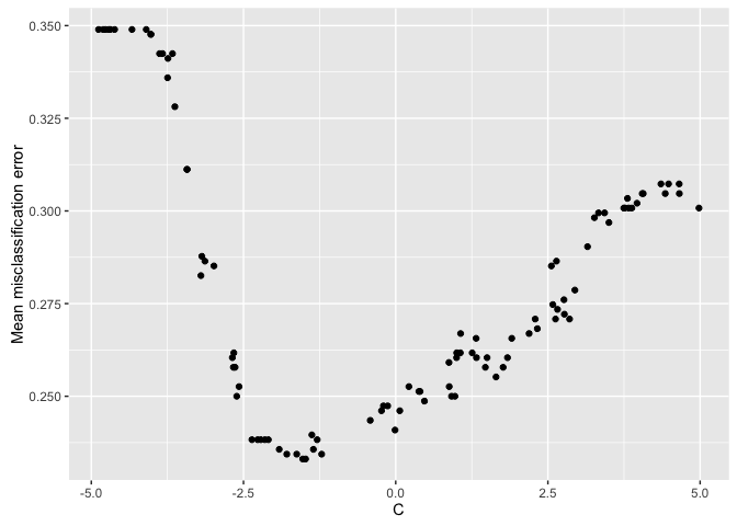
From the scatterplot, it appears our optimal performance is somewhere in the
region between 2^-2.5 and 2^-1.75. This could provide us a region to further
explore if we wanted to try to get even better performance!
We could also evaluate how “long” it takes us to find that optimal value:
plotHyperParsEffect(data, x = "iteration", y = "mmce.test.mean")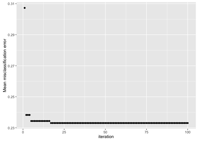
By default, the plot only shows the global optimum, so we can see that we found the “best” performance in less than 25 iterations!
But wait, I hear you saying. I also want to tune sigma, the inverse kernel
width of the radial basis kernel function. So now we have 2 hyperparameters that
we want to simultaneously tune: C and sigma.
# create the C and sigma parameter in continuous space: 2^-5 : 2^5
ps = makeParamSet(
  makeNumericParam("C", lower = -5, upper = 5, trafo = function(x) 2^x),
  makeNumericParam("sigma", lower = -5, upper = 5, trafo = function(x) 2^x)
)
# random search in the space with 100 iterations
ctrl = makeTuneControlRandom(maxit = 100L)
# 3-fold CV
rdesc = makeResampleDesc("CV", iters = 2L)
# run the hyperparameter tuning process
res = tuneParams("classif.ksvm", task = pid.task, control = ctrl,
  resampling = rdesc, par.set = ps, show.info = FALSE)
print(res)
## Tune result:
## Op. pars: C=0.233; sigma=0.0386
## mmce.test.mean=0.232# collect the hyperparameter data
data = generateHyperParsEffectData(res)We can use plotHyperParsEffect to easily create a heatmap with both hyperparameters.
We get tons of functionality for free here. For example, mlr
will automatically interpolate the grid to get an estimate for values we didn’t
even test! All we need to do is pass a regression learner to the interpolate
argument:
plotHyperParsEffect(data, x = "C", y = "sigma", z = "mmce.test.mean",
  plot.type = "heatmap", interpolate = "regr.earth")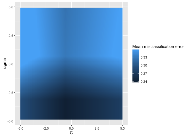
If we use the show.experiments argument, we can see which points were
actually tested and which were interpolated:
plotHyperParsEffect(data, x = "C", y = "sigma", z = "mmce.test.mean",
  plot.type = "heatmap", interpolate = "regr.earth", show.experiments = TRUE)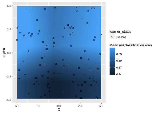
plotHyperParsEffect returns a ggplot2 object, so we can always customize it
to better fit our needs downstream:
plt = plotHyperParsEffect(data, x = "C", y = "sigma", z = "mmce.test.mean",
  plot.type = "heatmap", interpolate = "regr.earth", show.experiments = TRUE)
min_plt = min(plt$data$mmce.test.mean, na.rm = TRUE)
max_plt = max(plt$data$mmce.test.mean, na.rm = TRUE)
mean_plt = mean(c(min_plt, max_plt))
plt + scale_fill_gradient2(breaks = seq(min_plt, max_plt, length.out = 4),
  low = "red", mid = "white", high = "blue", midpoint = mean_plt)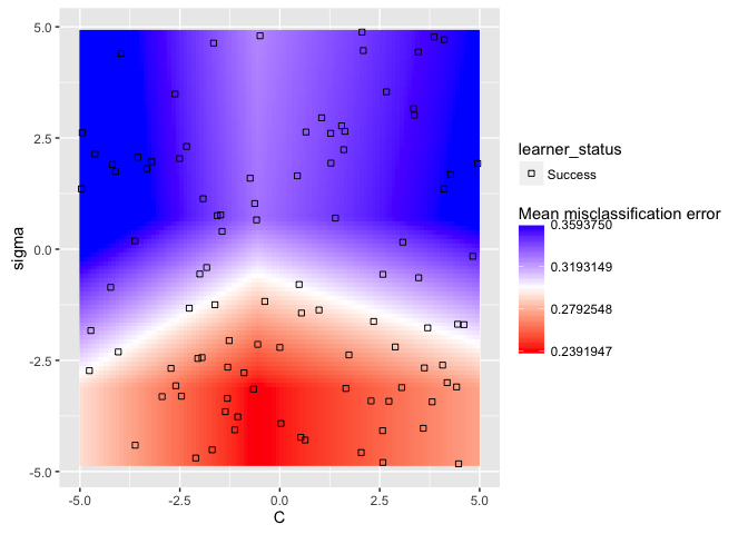
Now we can get a good sense of where the separation happens for each of the
hyperparameters: in this particular example, we want lower values for sigma
and values around 1 for C.
This was just a taste of mlr’s hyperparameter tuning visualization capabilities. For the full tutorial, check out the mlr tutorial.
Some features coming soon:
- “Prettier” plot defaults
- Support for more than 2 hyperparameters
- Direct support for hyperparameter “importance”
Thanks to the generous sponsorship from GSoC, and many thanks to my mentors Bernd Bischl and Lars Kotthoff!